Weather forecasts are an essential source of information for planning the day-to-day activities of our businesses. But how do we generate them? In this article, Damien Raynaud, meteorologist at FROGCAST, reveals the secrets of weather forecasting.
Collecting meteorological observations
Ground and altitude measurement networks
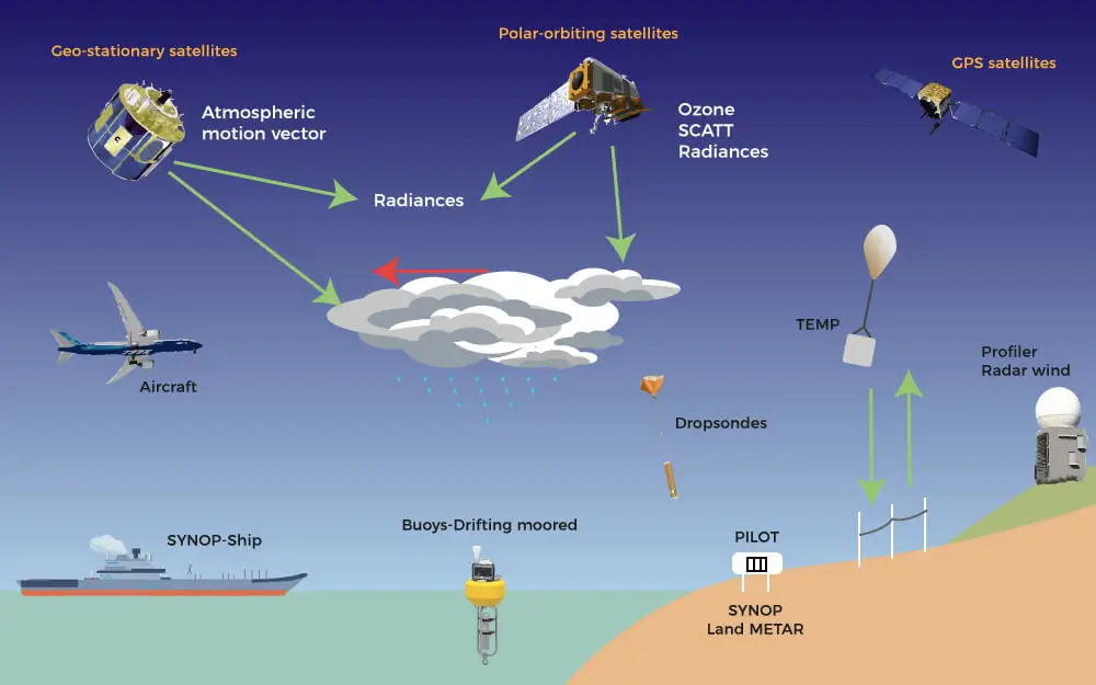
Forecasting the evolution of weather conditions over the coming days requires the most accurate possible knowledge of the current state of the atmosphere. For decades, we have developed networks of weather stations. They measure atmospheric parameters on the ground in real time.
Over time, other observation networks have supplemented these stations. They provide direct measurements at the ocean surface (weather buoys, sensors on boats) and at altitude (radiosondes, sensors on aircraft).
The era of meteorological satellites
But atmospheric observation has reached a new stage over the past 2 decades, with the launch of an ever-increasing number of high-performance meteorological satellites. They enable us to observe the atmosphere in a spatialized way. They estimate an ever-growing number of meteorological parameters on the ground, on the ocean surface and vertically in the atmosphere.
Other measuring instruments on the ground (radar and lidar) complement them, which also survey the atmosphere and provide precious information on clouds and precipitation.
Quality control of measurements
All sensors and associated measurements undergo continuous quality control. They must comply with standards that the World Meteorological Organization defines.
Did you know?
The COVID crisis between 2020 and 2022, and the associated reduction in air traffic and therefore in the weather observations that aircraft made, has had an impact on the quality of weather forecasts.
Numerical weather prediction models
The equations governing the atmosphere
The atmosphere obeys the equations of physics and thermodynamics, with the Navier-Stokes equation at its heart (we’ll spare you the details here 😭).
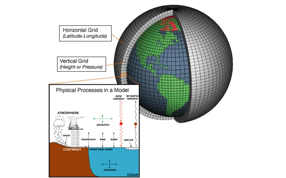
To simulate its evolution, we use mathematical models called Numerical Weather Prediction (NWP) models. In these models, we divide the atmosphere into cubes. Within these cubes, we consider the weather parameters to be homogeneous (a single value for temperature, humidity, etc.).
Model resolution
The horizontal and vertical dimensions of these cubes define the model’s resolution. The smaller they are, the better the model’s resolution. We call this division of the atmosphere the model grid.
Predicting the evolution of weather with these models involves solving these physical equations at every point on the grid and at every time. The finer the grid, the better the model simulates small-scale phenomena. It also represents in detail the atmosphere and surface characteristics (e.g. topography).
As we’ll see a little later, this comes with consequences for calculation resources. The higher the resolution, the greater the calculation power required to carry out the forecast.
Global and regional models
Every major meteorological center develops its own forecasting models. Some are global. They provide forecasts for every point on the globe. Others are regional. They calculate only for a specific area.
Spatio-temporal resolutions, forecasting timescales and update frequencies also differ from one model to another. We call each new simulation, generally carried out every 3 to 6 hours, a run.
Did you know?
There are several dozen operational weather models in the world today. However, only less than 10 of these are global.
The weather forecasting process
Data assimilation
To carry out its calculations and predict the evolution of the weather, we need to provide the model with a detailed description of the current state of the atmosphere at each of its grid points. This is where previously collected meteorological observations come into the equation.
We use a technique known as data assimilation. It generates an initial state of the atmosphere by merging information from the model’s previous run (e.g. the H+6 forecast from the run made 6 hours earlier) and observations made since then. The result is a complete 3D map of the atmosphere. It takes advantage of the direct and indirect weather measurements available since the last forecast.
Running the calculations
Now the calculations can start! At each grid point and time step, the model has to solve a set of complex equations. These are very costly in terms of computing resources.
Calculations generally take a few tens of minutes. This is thanks to the use of supercomputers. They can perform an impressive number of operations per second. For example, the latest supercomputer that Météo-France uses, commissioned in 2021, has no fewer than 300,000 cores. They can perform over 20 million billion operations per second.
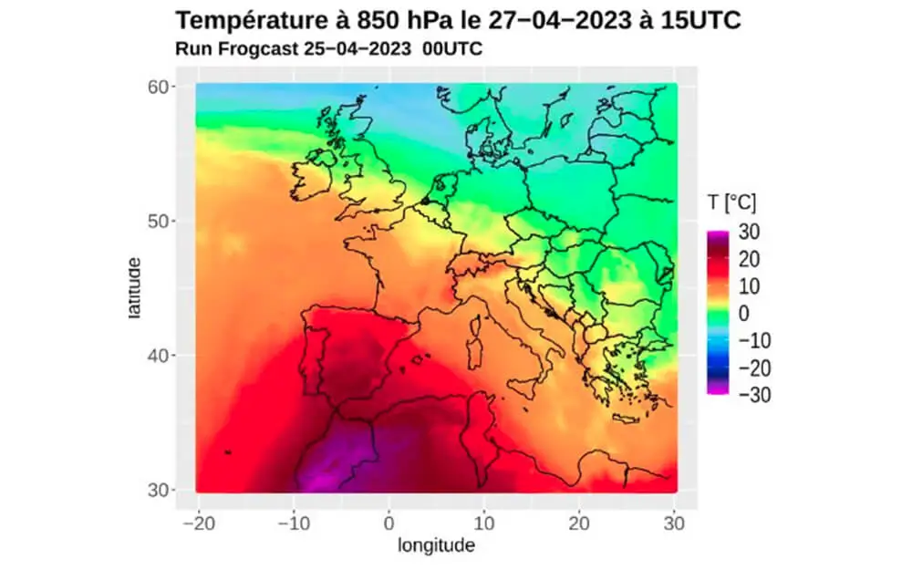
The final output is a 4D forecast (latitude, longitude, altitude and weather) of atmospheric trends over the coming hours and days.
Did you know?
Supercomputers look like a succession of cabinets from the outside. They contain calculation processors and are stored in a room measuring several dozen square meters. The heat that these operations generate is such that hydraulic cooling circuits are required.
Forecast reliability and chaotic atmosphere
The limits of predictability
Over the last three decades, the available calculation capacity has multiplied by more than ten million. In addition, networks of observations are becoming ever denser. They enable us to feed models with high-quality data. Our understanding of the physical processes involved in the atmosphere has also greatly evolved thanks to scientific research in this field.
So why do forecasts sometimes still face questions about their reliability?
The butterfly effect
In the early 1970s, Edward Lorenz developed an extremely simplified meteorological model to qualify the atmosphere’s behavior. His experiment consisted in feeding this model with two extremely close initial states. He then ran his calculations and compared the meteorological trajectories derived from these starting points.
The results showed something remarkable. After just a few iterations of the model, the two trajectories began to diverge significantly. They finally depicted two completely different states of the atmosphere.
Lorentz had just proved the chaotic nature of the atmosphere. He presented his results at a conference in 1972 with the now famous title: “Predictability: can the flapping of a butterfly’s wings in Brazil cause a tornado in Texas?“. The famous butterfly effect was born.
Managing uncertainty
This study illustrated the extremely complex behavior of the atmosphere. Inaccuracies in the initial state provided to the model, even the smallest ones, or in the modeling of very small-scale meteorological processes such as turbulence, inevitably lead to errors. These errors spread throughout the forecast and increase as the simulation runs.
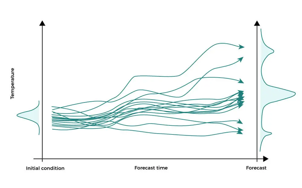
Fortunately, meteorologists have more than one string to their bow. They have learned how to overcome sources of uncertainty. For example, they use what we know as ensemble forecasting. This takes Lorentz’s experiment to a larger scale.
Since it is impossible to perfectly describe the state of the atmosphere at every point, we will not run the meteorological model with a single initial state. Instead, we run it with a set of initial states. These take into account the uncertainty at points where no measurements are available.
This results in a large number of meteorological scenarios. We then use them to evaluate the most accurate forecast for the coming days. These techniques are extremely costly in terms of calculation time. They are now possible thanks to supercomputers.
Did you know?
With the continuous improvement of forecasting methods, a 5-day forecast today is as accurate as a 24-hour forecast in the 80s. Today, we consider weather forecasts to provide relevant information up to 8 to 10 days ahead.
FROGCAST’s multi-model approach
At FROGCAST, we’ve developed a unique multi-model approach that leverages the strengths of multiple forecasting systems simultaneously. Rather than relying on a single model’s output, we analyze and combine predictions from several leading global and regional models. This methodology allows us to identify areas of agreement and disagreement among different forecasting systems, providing crucial insights into forecast reliability.
Our specialty lies in translating this multi-model analysis into actionable confidence intervals. By understanding where models converge or diverge, we can quantify the uncertainty associated with each forecast and communicate it clearly to our clients. This means you don’t just receive a single weather prediction – you get a comprehensive assessment of how confident we are in that prediction, enabling better-informed decision-making for your business operations.
Whether you’re planning logistics, managing energy resources, or coordinating outdoor events, knowing not just what the weather will likely be, but how certain that forecast is, can make all the difference.
Want to learn more about how our multi-model approach and confidence intervals can benefit your business? Discover our weather forecast and confidence interval!