Confidence intervals are an essential source of information in weather forecasting. They make it possible to objectively quantify the uncertainty associated with a forecast.
Here we define confidence intervals, describe how we generate them and illustrate their possible uses. Before going any further, we recommend that you read our article about weather forecasting. Some concepts and notions will be repeated here without being explained again.
Deterministic and probabilistic forecasts
What is a deterministic forecast?
The adjective deterministic refers to a weather forecast for which only a single scenario is available. This means a single simulation from a single numerical weather prediction model. In this case, it is impossible to determine the confidence in the forecast.
This situation can potentially lead to large errors, especially for distant forecast timescales or for meteorological phenomena whose occurrence and location are particularly difficult to predict.
To overcome this limitation, it is possible to use ensemble forecasting, which propose a whole set of scenarios and allows us to deduce the most accurate evolution of the atmospheric state.
Generating forecast scenarios
There are several ways of generating this set of scenarios:
- Multi-model: Every National Meteorological and Hydrological Services (NMHS) in the world has its own numerical weather prediction model. They all provide different forecasts, which are as many possible scenarios.
- Multi-member: We saw in our previous article about weather forecasting that it was possible to take advantage of the chaotic nature of the atmosphere. We can also use the uncertainty about the initial state that the model provides. Here, we generate a set of forecasts from a set of equiprobable initial states.
- Multi-run: Most operational numerical weather prediction models generate a forecast every 3 to 6 hours. The most recent forecast is statistically more likely to be the most accurate. However, it can be useful to take into account the one or two previous forecasts.
- Spatio-temporal radius: For certain meteorological variables, location and timing are difficult to establish (e.g. precipitation). In these cases, it can be interesting to use not only the model grid point and time step of interest. We can also use surrounding points and previous and following time steps.
From ensemble forecasting to quantiles
Understanding quantiles
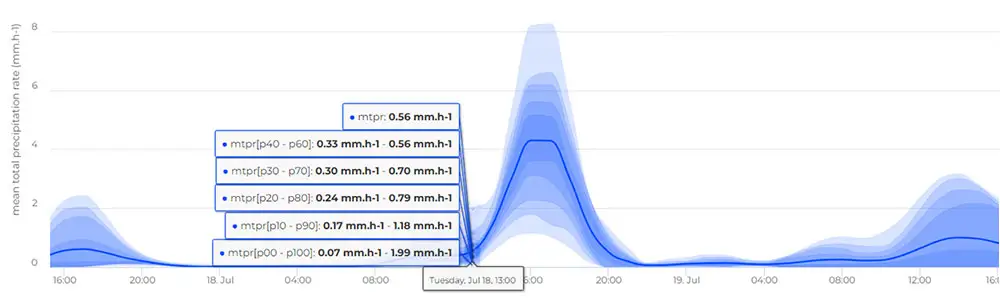
Now let’s imagine that we have at our disposal a very rich set of forecasts. It provides 100 scenarios of temperature forecasts at our point of interest. How do we process and take advantage of this data volume? Statistics!
For each time step, we will first sort our forecast temperature values in ascending order. We can then easily deduce quantiles. These divide our dataset into equiprobable intervals.
How quantiles work
For example, the 10% quantile (P10), is the expected temperature value such that 10% of our set is lower and 90% is higher. The 50% quantile (P50), also known as the median, is the temperature forecast such that 50% of our set is lower and 50% is higher.
What quantiles tell us
Quantiles provide essential information about the statistical distribution of our set. They therefore tell us about the confidence we can have in the forecast.
Example 1: High confidence
If our set gives a median value of 25°C, a P10 quantile of 24°C and a P90 of 27°C, this means that the set is relatively homogeneous. We have an 80% chance of having a temperature between 24°C and 27°C.
Example 2: Low confidence
On the other hand, if for the same median value of 25°C, the P10 and P90 quantiles are 17°C and 30°C respectively, this means that the different scenarios are widely dispersed and that the forecast is uncertain.
Case study: Frost risk in agriculture
The challenge of frost protection
Frost is one of the hazards most feared by farmers. The impact of frost on vineyards and orchards can be devastating if it occurs at flowering time. It can lead to a reduction or even total loss of harvests.
Producers invest a great deal of time, energy and financial resources in protecting their land against this hazard.
Protection methods
There are several ways to protect against frost:
- Sprinkling: This consists of irrigating parcels and covering buds with a layer of ice to keep them at a temperature close to 0°C.
- Atmospheric warming: Farmers use burners or heating wires.
- Air ventilation: Anti-freeze towers (also known as air blowers or helicopters) prevent the accumulation of cold air in the lower meters of the atmosphere.
All these techniques are very costly. It is essential to use high-quality meteorological measurements and forecasts to:
- Activate them when there is a risk of frost and avoid crop loss.
- Limit false alarms and thus avoid the costs associated with them.
A practical example
We propose here to use a simplified case to illustrate the contribution of quantiles in a temperature forecast. This will show how they help activate means to combat crop frost.
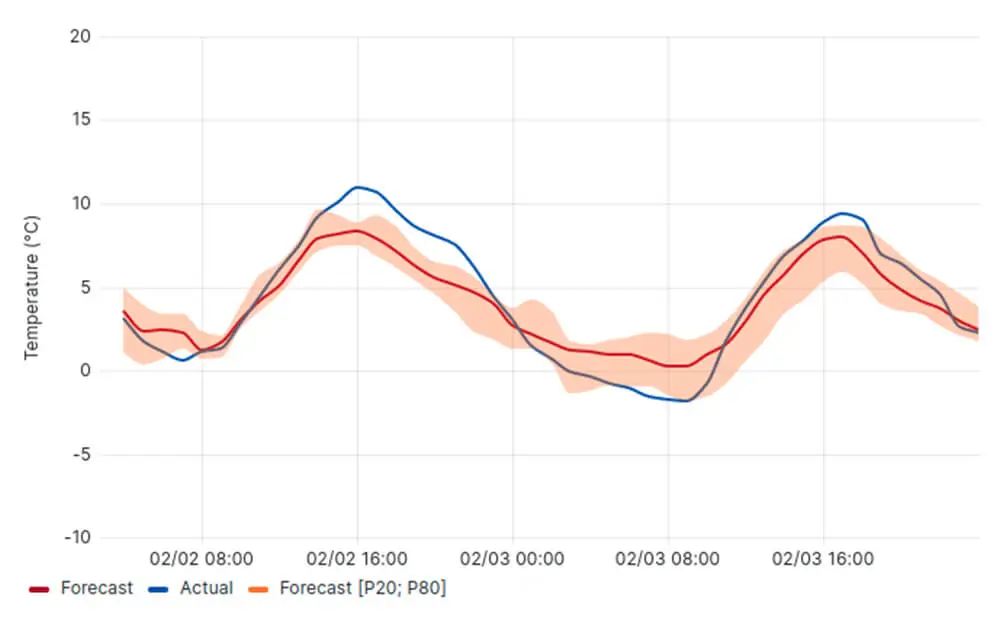
Let’s take the following temperature forecast for the next 48 hours for our point of interest. We assume that farmers will activate their frost protection measures in the event of a forecast indicating a temperature below 0°C.
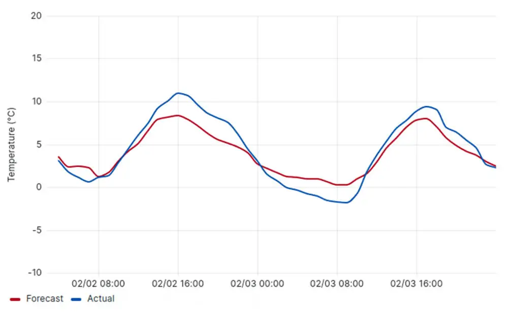
Scenario 1: Deterministic forecast only
In the first case, we only have a deterministic forecast (red). It does not indicate that the 0°C trigger threshold will be exceeded. Unfortunately, the temperature drops to -2°C on the second night. This causes crop damage.
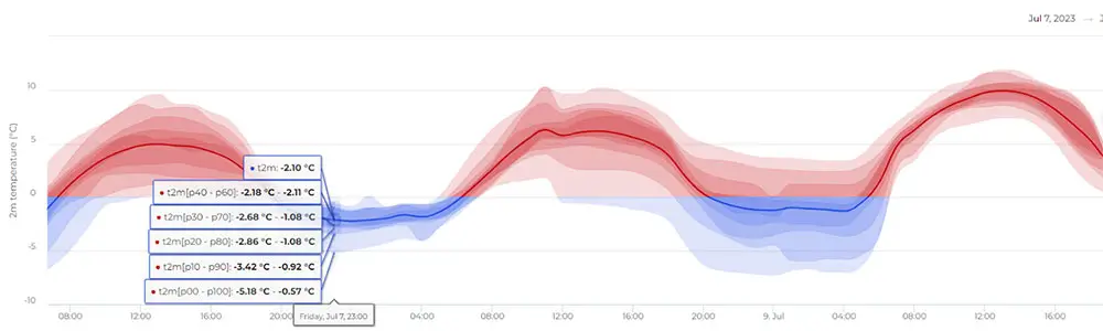
Scenario 2: Forecast with quantiles
In the second case, we also have two quantiles, P20 and P80, to quantify the confidence in our forecast.
On the first night, the P20 quantile also remains above 0°C. So it seems certain that the temperature will remain positive.
However, the uncertainty is higher for the second night. The risk of frost becomes significant.
Thanks to this information, the farmer will have been able to avoid activating his preventive equipment unnecessarily on the first night. But he will have protected his crops well on the second night!